Predicting deaths and hospitalization days in patients with neutropenia on MIMIC-IV using AI
16 Aug 2023In this post, we aim to leverage the data collected from the Medical Information Mart for Intensive Care (MIMIC-IV) version 4, a repository managed by the MIT Laboratory for Computational Physiology, which houses medical data for research purposes. This dataset, presented in [1], consists of patient information from the Beth Israel Deaconess Medical Center (BIDMC). Before accessing the dataset, ethical guidelines were followed as guided by the CITI Program course on Data or Specimens Only Research and the data usage was approved by the course instructor André Santanchè at the post-graduate discipline of Data Science and Visualization in Health at Unicamp. Our objective is to develop classification models for predicting mortality in neutropenic patients without cancer and regression models for predicting hospitalization days for patients with or without cancer.
This post was co-authored by Gustavo Luz and myself.
Wait. What is neutropenia and why it is relevant?
Neutropenia is one of the most concerning complications of chemotherapy and its prediction remains difficult [2] and this is when machine learning comes into place. If we can model this problem to early detect the possibility of dying and staying for a long time at the hospital based on the exams we can apply AI (artificial intelligence) to a critical disease and guide clinical treatment decisions [3].
⚠️ Important Statement: It is important to emphasize that although the problem was initially presented by a medical professional, the final results have not been reviewed by medical experts. Our team comprises computer science students and our primary aim is to showcase the application of data science tools to this issue. As such, this work serves as an illustrative example of how data science techniques can be applied to address challenges in the medical domain. It’s important to note that while our findings are presented here, no definitive medical conclusions should be drawn from this study.
Data preparation steps
Firstly, the dataset has been preprocessed and filtered to focus on patients with neutropenia, with steps documented that can be seen at this link.
After that, 10 steps were taken, the following being described:
- Removed rows with unidentified values in the ‘race’ column and rows with marital status ‘N’;
- Merged admission and diagnosis data using the Pandas library based on the ‘hadm id’;
- Created a new column indicating cancer diagnosis from the presence of “malignant neoplasm” in the diagnosis title. Added columns for related diagnoses based on expert insights and literature [4,5,6]. Removed duplicate rows;
- Filtered the dataset to include only the percentage of neutrophil count (item id 515256);
- Merged lab events and item descriptions based on the item id;
- Filtered the data to retain only relevant rows for the chosen lab test;
- Created new features by calculating mean, median, count, max and min values of exam results per admission. Removed duplicate rows;
- Merged admission, diagnosis and lab events data into a consolidated dataset;
- Removed undesired columns, checked for missing values, created columns for patient survival, hospitalization days and ensure data integrity;
- Conducted exploratory data analysis with visualizations to validate data treatment and gain insights into hospitalization days and neutrophil count distribution for patients with and without cancer.
Exploratory data analysis
Exploratory data analysis (EDA) is a crucial step in the data science process that involves visualizing and summarizing the dataset to gain valuable insights. During EDA, we examined various visualizations, including histograms and missing value distributions, to understand the data’s characteristics and identify potential patterns or trends. These visualizations validate the data’s integrity and allow us to make informed decisions for building predictive models and drawing meaningful conclusions about patient outcomes in cancer cases.
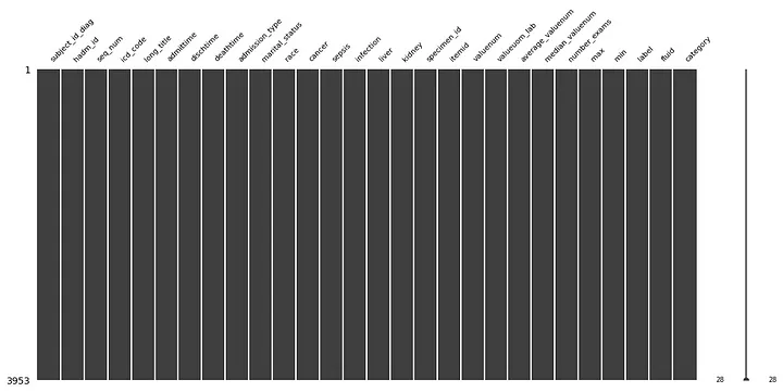
Missing values distribution: each column in this graph represents a variable and the absence of missing values (NaNs) results in continuous columns. The absence of missing data indicates effective data treatment.
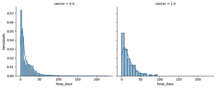
Hospitalization days histogram: this histogram presents the distribution of hospitalization days for patients with and without cancer. Patients with cancer show a higher concentration of hospitalization days, with the mode slightly shifted toward the right.
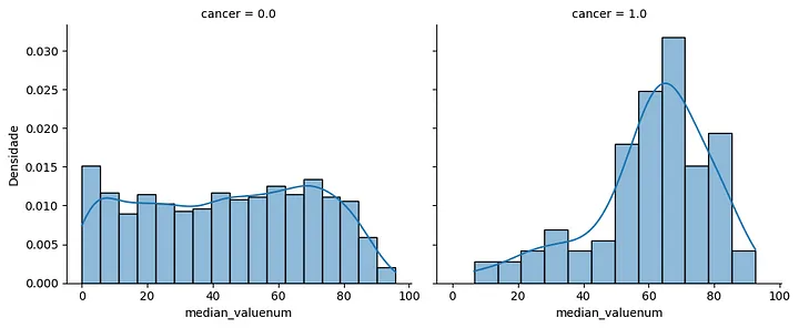
Median neutrophil count histogram: this histogram depicts the distribution of median neutrophil count values for patients with and without cancer. Patients with cancer exhibit a peak between 60% and 80%, while patients without cancer show a more evenly distributed histogram.
Modeling
To conduct the modeling process, we adopted the framework shown in the figure below:

Steps taken in the modeling phase.
Patient division by cancer status
Patients were divided into two subsets: those with cancer and those without cancer. These subsets were utilized for the classification and regression models with the corresponding selected features.
Correlation analysis
For better visualization than the traditional correlation matrix, a correlation graph was constructed.
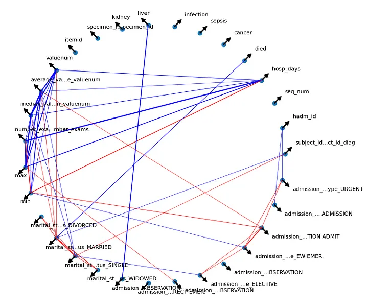
Correlation graph.
Blue lines indicate a Pearson correlation between pairs greater than or equal to 0.2 (positive low correlation), while red lines represent correlations less than or equal to -0.2. The line thickness reflects the degree of correlation, with thicker lines indicating stronger positive or negative correlations. Arrows denote each specific variable in the graph. Specific correlation analyses for each model type are discussed in the corresponding sections.
Steps Adopted in Modeling
Four steps were employed in the modeling process, including:
- Data Splitting (Train-Test Split): The data was split into training and testing sets using a random seed, with 70% for training and 30% for testing;
- Data Normalization: The data was normalized using Min-Max Scaling for the training set;
- Model Training: The models were trained, including a classification model to predict patient mortality and a regression model to predict hospitalization days for both cancer and non-cancer patients;
- Model Evaluation: The models were evaluated on the test set, using specific metrics for each case.
These steps were followed for both the regression and classification models, with the only difference being the option to perform class balancing for the classification problem of predicting patient mortality. Additionally, one-hot encoding was applied to the categorical variables before training the models.
Regression Models
A baseline model was developed to predict the number of days of hospitalization for patients with and without cancer. This baseline consists of a model based on linear regression. This simpler model was chosen to assess the ability of the regressor as well as its explainability.
To select the input features of the baseline model, the correlation between the preprocessed variables was analyzed as a selection criterion for those that made the most sense to be applied to the model. For example, the variable max presented a good correlation with the variable hosp_days (number of days the patient was hospitalized) and, therefore, was one of the selected variables.
Also observing the correlation graph, as input to the models, those variables were selected that presented a good correlation with the variable hosp_days and, on the other hand, a low correlation between the other pairs, in order to avoid a possible confounding factor between the input variables.
In this work, the evaluation metrics popularly applied to regression problems were used, namely: the coefficient of determination (R2), the mean absolute error (MAE), the root mean squared error (RMSE) and the mean squared error (MSE). Each of these metrics is briefly described below:
R2: indicates how much the regression model explains the variability of the data, ranging from 0 to 1;
MAE: Average of the absolute differences between the observed and predicted values by the model;
RMSE: Mean square root of the squared differences between the observed and predicted values by the model;
MSE: Mean squared errors between the observed and predicted values by the model.
The features selection criteria as well as the views described above were performed for each of the evaluated models: linear regression and artificial neural network. The results achieved in each of these models were aggregated in the table below.

Results obtained with the regressor for days of hospitalization.
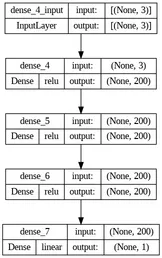
The architecture of the neural network used to build the regressors, which in this case was an MLP (multilayer perceptron), the number of neurons in each layer and their respective activation functions are shown in the figure below.
Classification Models
The classification modeling aimed to predict whether a patient would survive or not. The selected features for the models included hospitalization days, median exam values and marital status (divorced), following the same methodology as in the regression section.
There are patients with and without cancer. The focus of this work is to predict the second case, which showed a more significant sample to evaluate the model performance.
To address the complexity of the problem, traditional machine learning models such as logistic regression did not yield satisfactory results. Instead, the Random Forest model, which combines multiple decision tree results, was chosen as it showed promising results in various classification problems.
To improve performance, a Multilayer Perceptron Neural Network with one output neuron for binary classification was adopted. The network architecture included hidden layers with 19, 25, 98 and 8 neurons, regularization parameter alpha set to 0.03 and a maximum of 10,000 iterations.
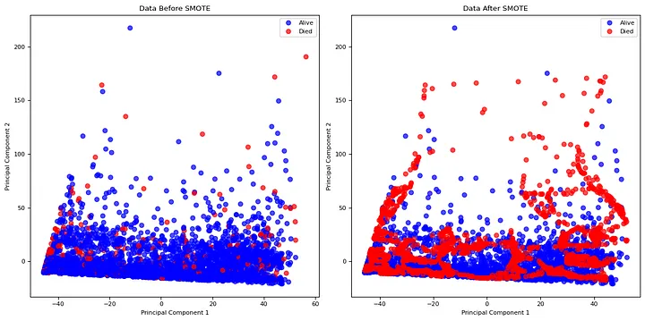
To address the class imbalance, the Synthetic Minority Oversampling Technique (SMOTE) was applied to the training set to generate synthetic samples for the minority class (deceased patients). This balanced the classes to have an equal number of samples for each classification.
Principal Component Analysis (PCA) with two components was performed for data visualization before and after balancing, providing a clearer understanding of the data, as shown by [7].
The evaluation metrics used for classification were accuracy, balanced accuracy and F1-score. Each of these metrics serves the following purpose:
Accuracy: Reflects the proportion of correctly classified instances among all instances in the dataset;
Balanced Accuracy: Represents the average accuracy achieved across different classes, compensating for class imbalances;
F1-score: Harmonic mean of precision and recall, offering a balanced assessment of model performance across different class distributions.
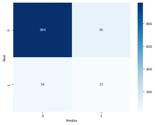
In the confusion matrix, the diagonal elements represent correct predictions, while off-diagonal elements represent misclassifications.
The balanced Random Forest model achieved an accuracy of 87.11%, indicating the percentage of correctly predicted outcomes out of all samples. The balanced accuracy, which takes into account both false positives and false negatives, reached 60.53%. This metric represents an overall balanced performance of the model, considering the class imbalance of the data. The model showed a better ability to distinguish between survival and death outcomes for patients without cancer compared to other tested models.
The best model was the balanced Neural Network, as shown in the table of results for non-cancer patients.

Results obtained with the classifiers for patients without cancer.
The Random Forest models exhibited poorer performance compared to the Neural Network and balancing had a positive impact only for the MLP model.
Conclusions and Future Works
Through this work, we conducted data treatments and visualizations that allowed us to model hospitalization time and mortality, creating relevant variables for prediction. We employed classical machine learning models and simple neural network techniques, considering the complexity of the problem.
In the classification task for predicting mortality in cancer patients, we encountered a low presence of deceased patients. Different data treatment strategies, such as generating multiple entries for each patient, were considered, but they may have drawbacks and require careful analysis. For non-cancer patients, the model showed better performance with a maximum balanced accuracy of 60.53%. Although this result might still be considered low for practical use, it can be improved using more advanced deep learning techniques, although with reduced interpretability.
For regression, predicting hospitalization days, the linear regression model achieved MAE values of 9.03 and 11.3 for patients with and without cancer, respectively. The neural network model achieved MAE values of 7.18 and 10.78 for patients with and without cancer, respectively. These values suggest relatively good predictions, with an average error of around one week. However, additional metrics assessing variance may be used for further evaluation.
Future work could involve creating new input variables using complete data versions, as this study utilized minimal datasets. Studies like [8] could provide insights into incorporating additional attributes, such as hemogram results containing hemoglobin, platelets, leukocytes, lymphocytes, monocytes, basophils, eosinophils and other relevant parameters, observing their correlations to improve model performance. All that mentioned are improvements that can be made to increase the number of patients that actually died, as the model learned well from patients that didn’t die. One approach to look is that the prediction of dying can be costly and it’s best to be more conservative in complex health problems.
⚠️ Ethics considerations: We underscore the ethical considerations in our classification and regression modeling approach for medical predictions. For future work, we recommend a deeper analysis of potential biases and disparities within historical data, particularly related to gender, race, and other protected characteristics. Additionally, implementing a robust system for ongoing monitoring is crucial to assess the ethical and equitable performance of these models over time. Exploring model interpretation methods is advisable to provide clearer insights into decision-making, thereby enhancing transparency and understanding. Furthermore, establishing protocols for disputes and appeals will enable individuals to question predictions perceived as unfair or inaccurate. These recommendations aim to strengthen the ethical integrity of future data science applications in the medical domain, fostering more equitable and informed decisions for patients and healthcare professionals.
References
[1] Johnson, A., Bulgarelli, L., Pollard, T., Horng, S., Celi, L. A., & Mark, R. (2021). MIMIC-IV. PhysioNet. Available at: https://physionet.org/content/mimiciv/1.0/
[2] Cho, B. J., Kim, K. M., Bilegsaikhan, S. E., & Suh, Y. J. (2020). Machine learning improves the prediction of febrile neutropenia in Korean inpatients undergoing chemotherapy for breast cancer. Scientific Reports, 10(1), 14803.
[3] Xiang, L., Wang, H., Fan, S., Zhang, W., Lu, H., Dong, B., & Fu, L. (2021). Machine learning for early warning of septic shock in children with hematological malignancies accompanied by fever or neutropenia: A single center retrospective study. Frontiers in Oncology, 11, 678743.
[4] Vaillant, A. A. J., & Zito, P. M. (2021). Neutropenia. In StatPearls [Internet]. StatPearls Publishing.
[5] Hosiriluck, N., Klomjit, S., Rassameehirun, S., Sutamtewagul, G., Tijani, L., & Radhi, S. (2015). Prognostic factors for mortality with febrile neutropenia in hospitalized patients. The Southwest Respiratory and Critical Care Chronicles, 3(9), 3–13.
[6] Perez-Figueroa, E., Álvarez-Carrasco, P., Ortega, E., & Maldonado-Bernal, C. (2021). Neutrophils: Many ways to die. Frontiers in Immunology, 12, 631821.
[7] Bahaweres, R. B., Salsabila, M., Rozy, N. F., Hermadi, I., Suroso, A. I., & Arkeman, Y. (2022). Combining PCA and SMOTE for software defect prediction with visual approach analytics. In 2022 10th International Conference on Cyber and IT Service Management (CITSM) (pp. 1–7). IEEE.
[8] Ferreira, P. L. & de Paula, E. V. (2020). The clinical and laboratory characterization of patients with febrile neutropenia from the MIMIC-III database. Available at: https://www.prp.unicamp.br/inscricao-congresso/resumos/2020P17753A13505O2527.pdf. Online; Accessed on June 6, 2023.